MLE-WorldOn this page

A learned world model for ML research

MLE-WorldPredicting Machine Learning Experiment Outcomes
with a Learned World Model

Brian Ko1 Han Wang2 Hejia Geng3 Li Erran Li4 Sherry Yang5
1University of Washington2University of Illinois at Urbana-Champaign
3University of Oxford4Columbia University5New York University

See the outcome. Before the run.

Highlights

Sample candidate programs, predict each outcome, then select, gate, and return feedback.

FIGURE 1(B)

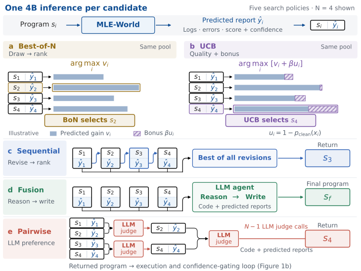
MLE-World enables test-time scaling

View paper figure ↗
Final submission: real runSelect the final program by its best real validation score.

Schematic from Figure 1(b): every candidate gets a predicted report before selection or combination. The returned program carries its MLE-World confidence into the gate; newly combined code receives a new prediction. Scores and the 0.80 threshold are illustrative. The full method also verifies new best predictions and uses outcome-specific thresholds.
Abstract

Machine learning research agents repeatedly write, run, and revise programs. Each real execution can require training and evaluation before the agent receives useful feedback. MLE-World predicts that execution feedback directly from code and task context: terminal output, an exception class, and a validation metric.

The learned predictor is a fine-tuned Qwen3.5-4B model. Research agents use its reports to screen, compare, or improve candidate programs, while a confidence gate determines when to request real execution. Final submissions are verified through real execution. The experiments below separately examine prediction fidelity, search quality, and real-execution cost.

Two roles for a learned world model

01 / PREDICT

Learn execution feedback

Turn candidate code, task data, environment, and runtime budget into a structured report. Compare those predictions with the outcomes of 1,700 held-out programs.

Explore prediction fidelity

How MLE-World guides search

Predict a report for each candidate, select or combine programs, then decide when real execution is needed.

World model performance

Prediction accuracy across four output fields, and the GPU time needed to predict execution outcomes.

1,700 held-out programs · 17 tasks
TABLE 1

Accuracy across prediction fields

In the paper ↗
Prediction accuracy in percent, with standard errors.
Model / baselineTerminal
output
Exception
class
Crash
class
Validation
metric
Prompted models
DeepSeek41.1 ± 1.157.2 ± 1.248.2 ± 1.518.6 ± 1.7
Coder17.8 ± 0.927.5 ± 1.113.2 ± 1.016.3 ± 1.7
Corpus, no model
Task majority—34.2 ± 1.2—55.2 ± 2.3
Nearest program28.0 ± 1.141.1 ± 1.214.0 ± 1.055.6 ± 2.2
Parent record22.3 ± 1.034.2 ± 1.26.7 ± 0.748.8 ± 2.3
MLE-World77.9 ± 1.086.4 ± 0.876.4 ± 1.378.1 ± 1.9

Scroll to compare all four prediction fields.

Accuracy (%); ± SE from 2,000 program bootstrap resamples. Exception class uses exact match; terminal output and crash class use judged match; validation metric is within 5% relative error. DeepSeek: DeepSeek-V4-Flash-0731. Coder: Qwen3-Coder-Next.
FIGURE 3

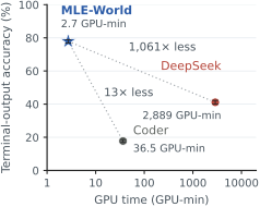
Accurate prediction at low inference cost

Full size ↗
Figure 3: terminal-output accuracy versus GPU generation time on a logarithmic scale. MLE-World: 77.9%, 2.7 GPU-minutes; Coder: 17.8%, 36.5 GPU-minutes; DeepSeek: 41.1%, 2,889 GPU-minutes.
Terminal-output accuracy versus GPU time (wall clock × GPUs; log scale). Bars: ± SE. Ratios use generation time for all models.

How reliable are the predictions?

Compare measured prediction fidelity with individual examples of what the model predicts and what actually happens.

1,700 held-out programs · 17 tasks
Loading the recorded evaluation…

FINAL RESULTS · FIGURE 1(C)

Final agent performance

Final solution quality versus real execution time across five MLE-World search policies under a 12-hour budget.

Open full size ↗
Figure 1c: Final quality and real execution from the 12-hour strict-score replay. Five MLE-World search policies are compared with Base AIDE. Open markers are ungated and filled markers use confidence gating; arrows show 32–40% less real execution, with higher observed mean percentile for all five policies.

Scroll to see the full chart, or open it full size.

Final quality and real execution. Mean leaderboard percentile of final solutions selected by the best real validation score. Each setting covers 17 tasks × three seeds (51 trials), with a 12-hour budget per trial and retrospective strict-score replay of fixed histories. The x-axis reports original mean elapsed time in real execution and recovery cleanup per trial, excluding inference. Open → filled markers show the change from ungated search to confidence gating: 32–40% less real execution and higher observed mean percentile for all five policies.

Same task. Different solutions.

Compare Base AIDE and five search policies on the same task. Inspect the strategies, saved programs, and independently graded outcomes.

2 tasks · all 6 policies

Higher percentile is better. Each score belongs to the saved program shown below, for run seed 34; it is not an average across seeds. Base AIDE uses the historical reference run.

Loading selected programs…

What changes

These examples were selected for different solution strategies and higher UCB than BoN percentiles in the displayed runs. Every task includes all six policies with the same run seed. TTS runs are ungated; see the aggregate results above for the overall comparison.

Explore other saved programs

For a closer look, choose any recorded task, seed, and pair of policies.

Compare two final programs

Selection used real validation scores. Private-test grades are shown only for evaluation.

Base AIDE is the same historical reference in both views. An unavailable or invalid final submission stays visible. Library labels are extracted from imports in the saved program.

Paper & resources

Read the paper, download the model and dataset, and explore the recorded evidence.